Original Article

Affiliation:
Eni S.p.A., 20097 Milan, Italy
Email: paolo.dell’aversana@eni.com
ORCID: https://orcid.org/0000-0002-0016-9469
Explor Digit Health Technol. 2024;2:218–234 DOI: https://doi.org/10.37349/edht.2024.00023
Received: March 18, 2024 Accepted: August 02, 2024 Published: August 15, 2024
Academic Editor: Gaurav Pandey, Icahn School of Medicine at Mount Sinai, United States
The article belongs to the special issue Deep Learning Methods and Applications for Biomedical Imaging
Aim: This study represents preliminary research for testing the effectiveness of the Self-Aware Deep Learning (SAL) methodology in the context of medical diagnostics using various types of attributes. By enhancing traditional AI models with self-aware capabilities, this approach seeks to improve diagnostic accuracy and patient outcomes in medical settings.
Methods: This research discusses an introduction of SAL methodology into the medical field. SAL incorporates continuous self-assessment, allowing the AI to adjust its parameters and structure autonomously in response to changing inputs and performance metrics. The methodology is applied to medical diagnostics, utilizing real medical datasets available in the public domain. These datasets encompass a partial range of medical conditions and diagnostic scenarios, providing an initial test background for a preliminary evaluation of the effectiveness of SAL in a real-world context.
Results: The study shows encouraging results in enhancing diagnostic accuracy and patient outcomes. Through continuous assessment and autonomous adjustments of its own neural network architecture, self-aware AI systems show improvements in adaptability, in the classification of real datasets and diagnostic process. Additional experiments on expanded data sets are necessary for validating these preliminary results.
Conclusions: Tests on real data show that Self-Aware Deep Neural Networks present promising potential for improving medical diagnostic capabilities. They offer advantages such as enhanced adaptability to varying data qualities, improved error detection, efficient resource allocation, and increased transparency in AI-assisted diagnoses. However, considering the limited size of the test data set used in this research, further validation is required through additional experiments on larger data sets.
The concept of self-awareness, once confined to the realm of human cognition and biological consciousness, is now expanding its horizons to encompass artificial agents and machines. In the domain of artificial intelligence (AI) and robotics, self-awareness denotes the hypothetical capacity of machines and artificial agents to introspectively perceive and understand their own operations, capabilities, and limitations [1–7]. This area of research holds significant promise across various disciplines, ranging from geosciences to financial and medical fields. In fact, self-awareness in machines offers a wide range of potential benefits, although it also presents its own set of challenges and limitations. By empowering artificial agents with rudimentary forms of self-awareness, we aim to enhance adaptability, robustness, and efficiency of artificial neural networks across diverse applications. For instance, in geosciences, self-awareness enables AI systems to adapt autonomously to dynamic environmental conditions, improving the accuracy and reliability of geological/geophysical models, data classification and probabilistic predictions of the dynamics of complex geological systems. In recent years, we have explored the integration of rudimentary self-awareness and self-reflection mechanisms into artificial deep neural networks, leading to notable advancements in tasks such as mineralogical microscope image recognition, rock classification, and other geological/geophysical disciplines [8–10]. Like their applications in the Earth Sciences, advanced AI systems can also enhance imaging and diagnostic accuracy in the medical field. Indeed, innovative analytical approaches have been proposed by various researchers over the past few years. For example, physics-driven personalized federated learning method (HyperFed) for CT imaging [11], is an effective approach based on the assumption that the optimization problem for each imaging domain can be divided into two subproblems: local data adaptation and global CT imaging. These are addressed by an institution-specific, physics-driven hypernetwork and a global-sharing imaging network, respectively. The main goal of the global-sharing imaging network is to learn stable and effective invariant features from diverse data distributions. Inspired by the physical process of CT imaging, a physics-driven hypernetwork is defined for each domain to derive hyperparameters from specific physical scanning protocols, conditioning the global-sharing imaging network to achieve personalized local CT reconstruction. Experiments demonstrate that this method delivers competitive performance compared to several state-of-the-art methods.
An additional approach recently introduced is based on a hybrid learning paradigm called Dynamic Corrected Split Federated Learning (DC-SFL) for U-shaped medical image networks [12]. In order to ensure data privacy, including the input, model parameters, labels, and output, the network is split into three parts, each hosted by different parties. The authors propose a Dynamic Weight Correction Strategy (DWCS) to stabilize the training process and prevent model drift due to data heterogeneity. To further enhance privacy protection and establish a trustworthy distributed learning paradigm, additively homomorphic encryption is introduced into the aggregation process of the client-side model. This approach helps prevent potential collusion between parties and provides a stronger privacy guarantee for the method. DC-SFL has been tested and evaluated on various medical imaging tasks, and the experimental results demonstrate its effectiveness compared to state-of-the-art distributed learning methods.
In the frame of innovative AI and machine learning methods applied in medical sciences, this paper introduces self-aware AI into the realm of medical diagnosis. Our basic assumption is that, where precise and timely diagnosis is paramount, self-aware AI systems can autonomously adapt to varying data qualities, patient demographics, and clinical contexts. By evaluating the confidence and reliability of their diagnostic outputs, these systems can assist radiologists and clinicians in making more informed decisions, leading to improved patient care and treatment planning. In the next sections, first we recall the key methodological aspects of the Self-Aware Deep Learning (indicated, briefly, with “SAL”). Then we apply this approach to a data set available in the public domain to test its effectiveness for solving real diagnostic problems.
The SAL methodology integrates adaptive learning and self-monitoring mechanisms within the field of AI, presenting a comprehensive framework aimed at enhancing the performance and adaptability of deep neural network models. Adaptive learning [13–15], a fundamental aspect of this methodology, enables computer algorithms and AI systems to customize learning experiences according to the specific requirements of individual learners, whether they are human or artificial agents. When applied to artificial neural network models, we redefine adaptive learning with a slightly different focus. This involves the deep neural network’s ability to readapt itself and adjust its internal architecture to accommodate specific datasets and address unique problem-solving challenges, while also considering the dynamic nature of the problems themselves. In our approach, adaptive learning is succinctly and effectively expressed through the following iterative formula, which is aimed at updating the model’s parameters and architecture based on feedback obtained from the learning process:
In this formula, introduced in a recent paper [8],
Through continuous self-assessment, the model gains insights into its performance trajectory, facilitating adaptive adjustments to improve learning. Automatically, the network model updates its complete functional structure by deducting the scaled gradient, allowing it to modify its internal representations based on feedback from the loss function. It is crucial to understand that, in a typical deep neural network, the loss function provides the difference between the predicted and true outputs. This function measures the model’s error or “loss,” indicating its performance level. One commonly used loss function is the mean squared error, while another prevalent choice in deep neural networks is the cross-entropy loss function. This latter one is frequently employed in classification tasks, where the aim is to assign input data to distinct categories or classes. The expression for the cross-entropy loss function in a multi-class classification case is:
where:
L represents the cross-entropy loss.
∑ denotes the summation over all N classes.
yi is the true label of class i (0 or 1 depending on whether the sample belongs to that class or not).
pi is the predicted probability of class i.
In the SAL approach, the learning rate α controls the step size of both the parameters and hyper-parameters updates. A higher learning rate allows for larger adjustments, while a lower learning rate ensures smaller, more cautious updates. Hence, the loss function also depends on the entire architecture Ω. The gradient
Here, P(t;Ω) represents the performance measure at time step t (epoch), for a given parameters and hyper-parameters set, Ω. The performance measure can vary depending on the task and the desired evaluation criteria. In classification tasks, a frequently used performance metric is the training and/or validation accuracy, which indicates the proportion of correctly classified or predicted samples. On the other hand, in regression tasks, the mean squared error is commonly employed as the performance metric, measuring the average squared difference between predicted and target values. The self-monitoring function M(O(t;Ω)) encapsulates the calculation of the performance measure. It takes the model’s output O(t;Ω) as its input and computes the desired performance metric.
In essence, through the integration of self-monitoring mechanisms, SAL enables neural networks to assess and enhance their performance iteratively, leading to advancements in adaptability and effectiveness. While this approach falls short of constituting genuine self-awareness as observed in biological entities, it does represent an effort to incorporate basic mechanisms of self-monitoring and adaptive behavior into deep neural networks. The objective is to enhance the architecture of the entire networks autonomously, without requiring human intervention.
In this subsection, we introduce the key technical details of SAL-type neural networks. As stated earlier, a critical aspect of SAL is the ability to perform a continuous “Internal State Monitoring”. This involves the implementation of mechanisms within the neural network architecture able to monitor neuron activations and the flow of information through neural layers. These mechanisms provide the network with basic control over its activity through continuous, autonomous analysis of fundamental hyper-parameters. For instance, “Neuron Activation Monitoring” allows tracking and logging the activations of neurons during both training and inference phases. This is done by adding “callbacks” that record the activation values of layers or specific neurons. Furthermore, the network itself continuously updates its internal statistics such as mean, variance, and distribution of activations. This helps in identifying abnormal patterns or saturation in neurons, which can signal the need for adjustments. Also, histograms of neuron activations are created and updated in order to visualize the distribution of activations across different layers.
Important benefits of all these implementations include, for instance, detecting vanishing or exploding gradients, identification of “dead neurons” (neurons that output the same value regardless of the input), and so forth.
Information Flow Tracking is another crucial functionality implemented in SAL. This is done through continuous Gradient Flow Analysis. This implies monitoring the flow of gradients during backpropagation to ensure that gradients are appropriately flowing through the network. This can be done by visualizing gradient magnitudes layer by layer. Furthermore, the SAL is able to self-control its own performances through “Intermediate Outputs Logging”: This allows to capture and store intermediate outputs (feature maps) from different layers. This helps in understanding how information is transformed at each epoch.
Performance Self-Evaluation is an additional fundamental step implemented in SAL. This encompasses mechanisms that allow the neural network to evaluate its own performance and recognize errors. Techniques such as loss prediction and confidence estimation assess the network’s uncertainties in its predictions and identify potential convergence issues.
Another key aspect is the implementation of rudimentary “self-reflection mechanisms”, also known as self-supervision or self-training, which enhance learning and performance by introducing additional tasks or objectives to the training process. This improves the network’s representation learning and generalization abilities.
Self-reflection mechanisms include Auxiliary Classifiers, Adaptive Loss Weights, and Adaptive Gradient-Based Regularization (AGBR). Auxiliary Classifiers are inserted at intermediate layers of the main network, predicting the same categories from different representations of the input data. This distributed learning approach improves generalization and robustness. Adaptive Loss Weights allow the model to assign different weights to losses from the main and auxiliary classifiers.
AGBR combines gradient-based optimization and adaptive regularization, dynamically adjusting regularization strength during training based on gradient information. This prevents overfitting by balancing model complexity reduction and pattern preservation in the data. Additionally, the SAL workflow iteratively adjusts hyper-parameters like Dropout, which prevents overfitting by creating subnetworks within the main network, and Momentum, which speeds up convergence and overcomes local minima during optimization.
Additional Advanced Neural Functions include specialized modules, such as attention mechanisms, that enable the network to focus on specific aspects of its internal state or the environment. Other functions are pre-processing self-optimization, automatic feature extraction, feature ranking, and optimal data normalization. Pre-processing tasks prepare input data before feeding it into the neural network, such as resizing images to a standard size, normalizing pixel values, or applying data augmentation techniques to increase training diversity.
Finally, we remark that illustrative tutorial codes in Python describing key steps of the SAL workflow are mentioned at the end of the paper (Supplementary material).
An important challenge in Self-Aware Deep Neural Networks is related to the update of some type of hyperparameters characterized by a discrete nature. In that case, the backpropagation techniques can show severe limitations. However, there are alternative techniques and strategies that can be employed to manipulate these discrete hyperparameters effectively. In our SAL architecture, we include several approaches, such as Hyperparameter Space Exploration Techniques. For instance, we apply a Bayesian Optimization approach that uses a probabilistic model to estimate the performance of hyperparameters and guides the search for optimal values. First, the network builds a surrogate model (e.g., Gaussian Process) to predict the performance of hyperparameters based on past evaluations. Next, the SAL network applies an acquisition function to balance exploration and exploitation in the hyperparameter space. Finally, SAL iteratively proposes new hyperparameters, evaluates them, and updates the surrogate model.
An alternative approach implemented in the SAL model is based on Grid Search method. This exhaustively searches through a manually specified subset of the hyperparameter space. Multiple models with different hyperparameters are trained in parallel, and poorly performing models are periodically replaced and mutated based on the performance of the better ones. It is sometimes effective, but in many cases can be very time consuming.
An additional approach includes Adaptive Hyperparameter Tuning Techniques that maintains a population of models with different hyperparameters and periodically evolves them based on performance.
In summary, in the SAL workflow, we have the possibility to select one or more of the above approaches, depending on the nature of the problem to solve and on the size of the data set. By implementing one or more of these techniques in parallel, a self-aware neural network can dynamically adjust its hyperparameters during training, optimizing its performance more effectively than static hyperparameter settings.
At the end of this paper, we included the simple tutorial code illustrating the key steps for updating hyperparameters having discrete and/or non-numerical nature (Supplementary material).
After having explained the key technical details about SAL architecture and how the SAL model updates (continuous as well as discrete) hyperparameters, in this sub-section we can schematically describe how the SAL model can be applied in practice.
Figure 1 illustrates the primary components of the SAL workflow. On the left side of the diagram, we can observe “standard” networks like convolutional or residual networks [16–18], which initially process input data according to specific tasks. These networks generate an initial output, such as image dataset classification or time-series data prediction. By continuously evaluating network performance, all essential hyperparameters are monitored autonomously by the network itself. The objective is to evaluate the network’s performance in real-time without external user intervention and adjust the network’s architecture to improve results. This involves maximizing accuracy criteria while simultaneously minimizing the validation loss function to mitigate overfitting effects. Performance is compared continuously to previous results, and hyperparameters are adjusted accordingly (see eq.1). This process continues until one or more stopping criteria are met. These criteria can be, for instance, maximum number of iterations, convergence of hyperparameters below a predefined threshold, stationarity in performance improvement, resource constraints, and so forth.
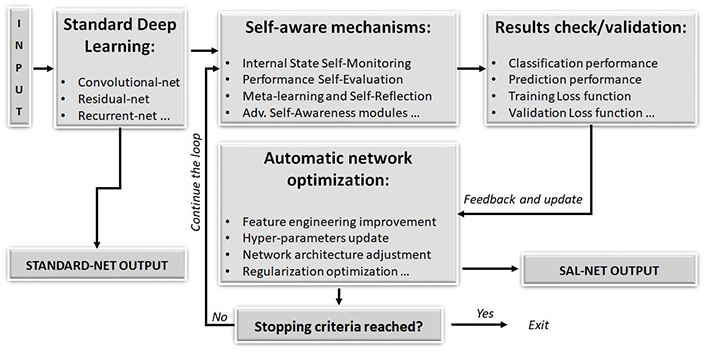
Block diagram of the SAL architecture and workflow
Note. Reprinted from “Enhancing Deep Learning and Computer Image Analysis in Petrography through Artificial Self-Awareness Mechanisms” by Dell’Aversana P. Minerals. 2024;14:247 (https://www.mdpi.com/2075-163X/14/3/247). CC BY.
In the upcoming section, we are going to apply this workflow to actual datasets sourced from medical imaging for diagnostic purposes. We will perform a comparative analysis between the SAL approach and traditional neural network models, along with alternative algorithms employed on identical datasets. This comparative assessment seeks to clarify the strengths and weaknesses of the SAL methodology when juxtaposed with other well-established machine-learning techniques.
We remark that, in this article, we limit the application of the SAL approach to a single real dataset (although we included the links to additional tests on synthetic data). Indeed, this paper aims to introduce the SAL methodology in the medical field. Therefore, it is primarily focused on the methodological description of our approach. This implies that further tests and more in-depth analyses will be necessary to validate the effectiveness of Self-Aware Deep Neural Networks more confidently. Despite these experimental limitations, we remark that in previous papers, we have already described additional examples of applications of the SAL approach in fields other than medicine. For instance, in some recent works, we have demonstrated the benefits of this approach in the fields of geosciences, hydrocarbon exploration, and drilling engineering [8–10].
Medical imaging and medical diagnosis, with their diverse modalities and complex datasets, often encounter challenges related to data variability, noise, and dynamic conditions. By developing deep neural networks with basic self-awareness capabilities, we can address these challenges and unlock several potential advantages.
One significant benefit lies in the realm of improved adaptability. Our work-hypothesis is that artificial neural networks equipped with rudimentary self-awareness mechanisms can autonomously adjust their hyper-parameters and architectures in response to changing conditions, such as evolving datasets or dynamic patient characteristics. This adaptability is particularly pertinent in medical sciences, where patient data may exhibit temporal variations or imbalances across different demographic groups.
Furthermore, integrating self-awareness mechanisms can enhance error detection and handling within medical imaging/diagnosis tasks. Neural networks endowed with self-awareness can evaluate the confidence and reliability of their predictions, enabling more robust decision-making processes. In medical diagnostics, where accuracy is crucial, this capability can facilitate the identification of uncertain or ambiguous cases, thereby improving patient care outcomes.
Efficient allocation of computing resources is another key advantage offered by self-aware neural networks in medical applications. By dynamically assessing the complexity of tasks, these networks can optimize resource allocation, prioritizing computations for accurate diagnoses or image reconstructions. This efficiency gain is particularly significant in resource-intensive medical imaging modalities, such as MRI or CT scans, where timely analysis is essential for patient management.
Furthermore, self-awareness mechanisms enhance the explainability of neural network outputs in medical applications. By providing insights into the decision-making process, these mechanisms make the models more interpretable for clinicians and radiologists. This transparency fosters trust in AI-assisted diagnoses and facilitates collaboration between healthcare professionals and AI systems.
In summary, the integration of rudimentary self-awareness and self-reflection mechanisms into artificial neural networks holds high potential for advancing medical imaging/diagnostic capabilities. In the subsequent sections, we will delve into the pragmatic aspects of SAL, introduce it through synthetic data tests, and finally, apply it to real medical imaging datasets, elucidating its practical benefits and limitations in clinical settings. However, we want to emphasize that the test results discussed in this article should be considered with caution. The experimental data set used here is, in fact, limited in size, and therefore further tests will be necessary to validate the SAL methodology in the context of medical diagnosis.
The conventional method for diagnosing breast tumors can involve a full biopsy, which is an invasive surgical procedure. Fine needle aspirations (FNAs) offer an alternative by allowing the examination of a small tissue sample from the tumor. However, as remarked by Street et al. [19], the success rate of diagnosis using this method, in some cases, can be low. Some specialized institutions have achieved successful diagnoses with FNAs by meticulously analyzing both the characteristics of individual cells and significant contextual factors, such as the size of cell clusters. Nonetheless, there is a belief that various features are associated with malignancy, making the diagnostic process often subjective and reliant on the expertise of the physician. To enhance the speed, accuracy, and objectivity of diagnosis, we can apply advanced image processing combined with machine-learning techniques. In the tests discussed in this section, we show how deep learning empowered by self-awareness mechanisms (SAL) can be successfully applied to an experimental data set of images (see below for details about the data) for significantly improving the reliability of the diagnosis.
The breast cancer databases used for the following test was obtained from the University of Wisconsin Hospitals, Madison [19, 20] (See the section “Availability of data and materials” for details).
Street et al. [19], and Bennett and Mangasarian [21], have employed advanced image processing techniques, coupled with a linear-programming-driven inductive classifier, to develop a precise system for diagnosing breast tumors. A small portion of a fine needle-aspirate slide is chosen and converted into digital format. Through an interactive interface, users initialize active contour models, referred to as “snakes”, near the perimeters of a group of cell nuclei. These “customized snakes” are then adjusted to precisely match the contours of the nuclei, facilitating accurate automated analysis of nuclear characteristics such as size, shape, and texture. Ten distinct features are computed for each nucleus, and the average value, maximum (or “worst”) value, and standard error of each feature are determined across the spectrum of individual cells. Following the analysis of 569 images in this manner, various combinations of features were experimented with to identify those that most effectively distinguish between benign and malignant samples.
We used these selected features for testing our entire SAL approach. In the following, we are going to explain, briefly, the key steps of our workflow addressed to a new binary classification of this experimental data set, based on our SAL machine-learning integrated platform. This includes a full set of algorithms (SAL plus complementary machine learning techniques) chained in effective workflows addressed to feature engineering, data processing and normalization, supervised and unsupervised classification, cross-validation tests and training, classification performance analysis and, finally, result mapping. For the entire workflow, we used a proprietary software platform. This has been designed and programmed by us “in-house”, using well-known Python libraries, such as Scikit-learn, SciPy, Keras/TensorFlow, Matplotlib, and so forth.
Feature engineering is the process of selecting, transforming, and creating new features from raw data to improve the performance of machine-learning models. It involves identifying and extracting relevant information from the input data that can help the model understand the underlying patterns and relationships. The following are some key aspects of feature engineering applied to this data set.
Feature Selection: This involves choosing the most relevant features from the available dataset. In this database, ten real-valued features are computed for each cell nucleus:
radius (mean of distances from center to points on the perimeter)
texture (standard deviation of gray-scale values)
perimeter
area
smoothness (local variation in radius lengths)
compactness (perimeter^2 / area – 1.0)
concavity (severity of concave portions of the contour)
concave points (number of concave portions of the contour)
symmetry
fractal dimension (“coastline approximation” – 1)
The mean, standard error and “worst” or largest (mean of the three largest values) of these features were computed for each image, resulting in 30 features. The class distribution is characterized by 357 benign, 212 malignant cases.
Feature Transformation: Sometimes, the distribution of the features in the dataset may not be ideal for the machine-learning algorithm. In our case, we applied feature transformation techniques, such as normalization, standardization, logarithmic transformation, and scaling. These can help make the features more suitable for classification.
Feature Scaling: Features with different scales and units can lead to biased model training and convergence issues. We applied feature scaling techniques, such as Min-Max scaling or Z-score normalization. These can help standardize the scale of features, ensuring that they contribute equally to the model’s learning process.
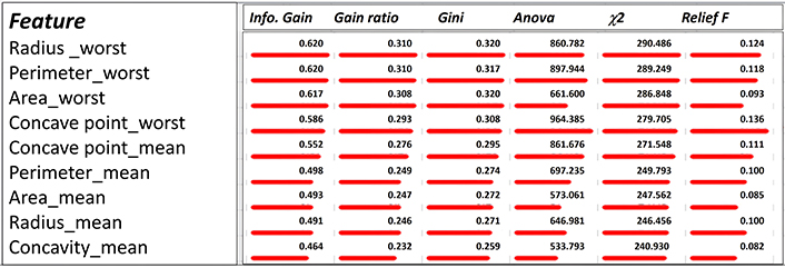
Feature Ranking: This step in the workflow helps in identifying the most relevant features for building machine-learning models, leading to improved model interpretability, reduced overfitting, and better generalization performance. Figure 2 shows an example of ranking for the first 9 features extracted from this data set. The length of the horizontal bar indicates qualitatively the relevance of the features for distinguishing benign from malign class using a pre-labelled data set (training sub data set). The ranking values have been extracted in a quantitative way, and are visualized in the table.
In the context of machine-learning feature ranking, the following terms are commonly used to assess the importance or relevance of features:
Info. Gain (information gain): This is a measure used in decision trees to quantify the reduction in entropy or uncertainty about the target variable achieved by splitting the data based on a particular feature. Higher information gain indicates that the feature effectively separates the data into classes, making it more informative.
Gain ratio: This is a variation of information gain; it takes into account the intrinsic information of a feature to avoid bias towards features with a large number of categories. It penalizes features with many categories.
Gini Index (Gini impurity): This is a measure of impurity or disorder used in decision trees. It quantifies the probability of incorrectly classifying a randomly chosen element if it were randomly labeled according to the distribution of labels in a particular node. Lower Gini Index values indicate that a node contains predominantly instances from a single class, making it a good split candidate.
ANOVA (analysis of variance): This is a statistical method used to compare means across multiple groups or categories to determine whether there are significant differences between them. In feature ranking, ANOVA is often used to assess the significance of differences in feature means across different classes or target variable categories. Features with higher ANOVA F-values are considered more important.
χ2 (Chi-square): This is a statistical test used to determine the association or independence between categorical variables. In feature ranking, χ2 is used to assess the significance of the relationship between a categorical feature and the target variable. Higher χ2 values indicate a stronger association between the feature and the target variable.
ReliefF (relief feature selection): This is a feature selection algorithm that evaluates the importance of features based on their ability to distinguish between instances of the same and different classes. It works by iteratively sampling instances and updating feature weights based on the nearest instances of the same and different classes. Features with higher weights are considered more important.
All the above indexes provide different perspectives on feature importance and are utilized in various machine-learning algorithms and techniques for feature ranking and selection. Each method has its strengths and weaknesses, and the choice of method depends on factors such as the nature of the data, the problem domain, and the specific requirements of the machine-learning task.
In the classification tests discussed in the following, we applied different neural network architectures as well as different alternative machine-learning algorithms, to compare their performances and select the optimal method(s) for our classification purposes. The effectiveness of different classifiers can vary depending on several factors, such as the characteristics and quality of the data and the nature of the classification problem. A robust approach to selecting the most suitable learning algorithms involves assessing their generalization performance and choosing the ones demonstrating the best results. One method for this selection process is conducting “cross-validation tests.” Cross-validation involves dividing the labeled data (the training dataset) into complementary subsets. The analysis is then performed on one subset (the training subset), and the results are validated on the other subset (the validation subset or testing subset). Various performance metrics are utilized to quantify the performance of each classification algorithm during cross-validation testing (as discussed below).
In machine learning, training a model involves using a subset of labeled data, known as the training set, to teach the model to recognize patterns and make predictions. Here is a step-by-step explanation of the workflow including training, classification of the remaining data (validation sub-data set, not included in the training sub-set), and evaluation of classifier performance. Let us start with the training phase. It includes the following sub-steps:
Data Preparation: The training subset of data is preprocessed and divided into input features (X) and their corresponding target labels (Y).
Model Initialization: An appropriate machine-learning algorithm is selected, and a model is initialized with random parameters.
Training: The model is trained using the training data by iteratively adjusting its parameters to minimize a predefined loss function. This is typically done through optimization algorithms like gradient descent, which update the model’s parameters based on the gradients of the loss function with respect to those parameters.
Loss Function Trends: Throughout the training process, the loss function is monitored to assess how well the model is learning. The goal is to see a decreasing trend in the loss function over epochs (training iterations), indicating that the model is improving its performance.
After the training phase, we apply one or more classifiers for the Classification Phase. It consists of the following main steps:
Data Preprocessing: The remaining part of the data (the validation or testing set) is preprocessed in the same way as the training data.
Prediction: The trained model is used to make predictions on the input features of the validation/testing set.
Classification: Each instance in the validation/testing set is assigned a predicted label based on the model’s output.
The final part of the workflow is the Evaluation Phase. It consists of the following main sub-phases:
Performance Parameters: Various performance metrics are calculated to evaluate the classifier’s performance. These metrics may include accuracy, precision, recall, F1 score, area under the ROC curve (AUC), among others. These metrics provide insights into how well the model is performing in terms of correctly classifying instances.
Loss Function Trends: The loss function trends observed during training are analyzed to ensure that the model has converged to a stable solution and is not overfitting or underfitting the data.
Scatter Plot Analysis: A scatter plot of the classified data can provide visual insights into the performance of the classifier. Different features are typically plotted on the axes of the scatter plot, allowing for visualization of the distribution of data points and how well they are separated into different classes by the classifier. This visualization helps in understanding the decision boundaries learned by the model and identifying any potential misclassifications or clustering patterns.
In the following section, we show how we applied the entire workflow using different methods. Our goal is to show how deep neural networks empowered with the SAL approach, perform better than “standard” deep neural networks and other machine-learning algorithms.
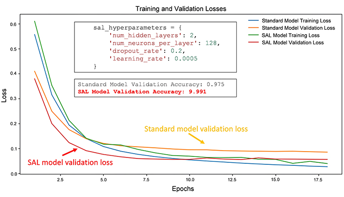
The first test consists of classification of a sub-set of validation data trained on a percentage of labelled data ranging from 50% to 90% of the entire data set. In this test, we compared the performances of the SAL network and Standard Deep Neural Network. Figure 3 shows an example of comparison of the training and validation losses for both types of methods. Both networks are initialized using two hidden layers and the same initial number of neurons for each layer and other hyper-parameters (such as the learning rate). However, different from the standard model, the SAL network can update dynamically (through the epochs) its own architecture and hyper-parameters to improve its classification performance and, at same time, avoiding overfitting problems. In this first test, the figure shows that the SAL model can obtain very high classification accuracy. Moreover, the validation loss curve (in red) converges towards values lower than that of the standard model (orange).
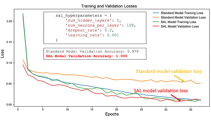
Comparison of losses curves of standard and SAL models for Test 1. In the upper box, the initial SAL hyper-parameters are shown; in the lower box, the final validation accuracies for both models are compared
The oscillations observed in the training accuracy trend of the SAL model (green curve) can be attributed to the iterative nature of the model’s architecture adjustments. In fact, the SAL model dynamically adjusts its architecture and hyper-parameters during training based on its performance on the validation set. This iterative process involves changing the number of hidden layers, the number of neurons per layer, the dropout rate, the learning rate, and other hyper-parameters. As a result, the model’s architecture evolves over time, leading to fluctuations in its performance metrics, including training accuracy. Furthermore, the iterative adjustments made to the SAL model’s architecture can introduce some level of instability during training. Each adjustment may cause the model to explore different architectural configurations, which can lead to variations in its learning behavior and performance. These variations can manifest as oscillations in the training accuracy trend.
Despite the oscillations, the SAL model aims to converge to an optimal architecture that maximizes its performance on the validation set. In summary, the oscillations in the training accuracy trend of the SAL model are likely a consequence of its iterative architecture adjustment process, which involves exploring different architectural configurations to improve performance. These oscillations reflect the dynamic nature of the SAL model’s learning process as it strives to adapt its architecture to the given dataset and task.
Figure 4 shows the final cross plot of the classified data (validation data set) using the SAL model. The plot is displayed for two specific features (radius_mean and concavity_mean), but the classification process used all the available features.
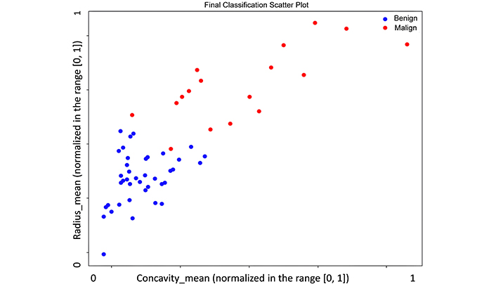
Classification cross plot for the SAL model for Test 1, with respect to two specific normalized features: radius_mean and concavity_mean
The second test is like the previous one. It has the same goal and allows a quantitative comparison between the performances of a standard neural network model and a SAL model. However, we changed slightly the initial hyper-parameters of the SAL model (such as the learning rate). Like in Test 1, in this case too, the SAL model performances are better than the standard model, although the accuracy is not 100%. This test is useful because it shows that a small difference in the initial parameters (in this case, the learning rate) can bring to variable final performances. However, the advantage of the SAL approach is that it can iteratively update its hyper-parameters and architectures with the objective to improve the performances and to optimize the classification results (optimal separation of the classes in the feature space, with reduced or null overfitting problems) (Figures 5, 6).
Comparison of losses curves of standard and SAL models for Test 2. In the upper box, the initial SAL hyper-parameters are shown; in the lower box, the final validation accuracies for both models are compared.
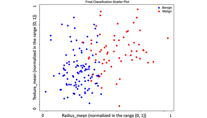
Classification cross plot for the SAL model for Test 2, with respect to two specific normalized features: radius_mean and texture_mean
Finally, we run a more comprehensive test for comparing the classification performance of the optimal SAL model(s) found through the previous tests and the performance of other machine-learning algorithms. These include Decision Tree, Random Forest, Logistic Regression, Naive Bayes and Support Vector Machine (SVM) (for a detailed explanation of these methods, see [16–18]).
As expected, all the methods perform well with this data set, but the SAL model shows the best performances. Table 1 shows the comparison between these methods in terms of performance parameters after cross-validation tests.
Performance comparison for different classification methods
| Method | AUC | CA | F1 | Precision | Recall |
|---|---|---|---|---|---|
| Tree | 0.925 | 0.928 | 0.928 | 0.928 | 0.928 |
| SVM | 0.992 | 0.952 | 0.951 | 0.955 | 0.952 |
| Random Forest | 0.986 | 0.950 | 0.950 | 0.950 | 0.950 |
| SAL Network | 0.997 | 0.994 | 0.994 | 0.994 | 0.994 |
| Naive Bayes | 0.983 | 0.934 | 0.934 | 0.934 | 0.934 |
| Logistic Regression | 0.927 | 0.929 | 0.929 | 0.929 | 0.929 |
AUC: area under the ROC curve; CA: classification accuracy
Let us explain, briefly, the performance indexes appearing in the table.
The “AUC” index, derived from “Area Under the Curve,” signifies the degree of separability and indicates a model’s capability to distinguish between classes. Higher AUC values suggest better predictive performance, particularly valuable in medical applications for distinguishing between patients with and without a disease.
Another crucial metric is the “Classification Accuracy” (CA), representing the proportion of correctly classified examples.
The “F1” score, a weighted harmonic mean of precision and recall, is also included. Precision measures the proportion of true positives among instances classified as positive, while recall assesses the proportion of true positives among all positive instances in the dataset.
Finally, to provide a general picture of the results of this binary classification test, Figure 7 shows an example of scatter plot obtained using the SAL model applied to an expanded validation data set.
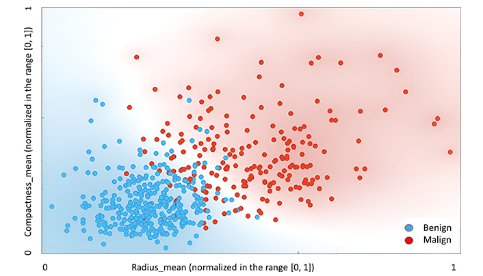
Classification cross plot for the SAL model for Test 3, with respect to two specific normalized features: radius_mean and compactness_mean
While the Self-Aware Deep Neural Network approach offers promising opportunities for enhancing medical imaging and diagnosis, addressing the associated challenges and limitations is crucial to realize its full potential in clinical practice. Continued research and development efforts focusing on improving model robustness, interpretability, and ethical considerations are necessary to ensure the responsible and effective deployment of AI technology in healthcare settings. We reiterate that the application of the SAL workflow in the medical field is still in its infancy. Additional efforts and tests are necessary to achieve full validation of this methodology. The following are some additional areas of research and possible improvements we are considering for enhancing our Self-Aware Deep Neural Network approach:
Dynamic Learning Rate Scheduling: Implementation of dynamic learning rate scheduling techniques such as “Reduce-LR-On-Plateau” or “Learning-Rate-Scheduler” to adjust the learning rate during training based on the model’s performance. This can help improve convergence and prevent overfitting.
Architecture Search Algorithms: Exploration of automated machine-learning (AutoML) techniques like neural architecture search (NAS) to automatically search for optimal network architectures. NAS algorithms can efficiently explore a large search space of architectures and find models that perform well on the given task.
Regularization Techniques: Experimenting with different regularization techniques such as L1 and L2 regularization, as well as techniques like dropout, batch normalization, and weight decay. These techniques can help prevent overfitting and improve the generalization performance of the model.
Ensemble Learning: Utilizing ensemble learning methods to combine predictions from multiple models trained with different hyper-parameters or architectures. Ensemble methods like bagging, boosting, and stacking can often lead to better performance than a single model.
Model Distillation: Applying “model distillation techniques” to transfer knowledge from a larger, more complex model (teacher model) to a smaller, simpler model (student model). This can help improve the performance of the student model by learning from the soft targets produced by the teacher model.
Transfer Learning: Investigating transfer-learning approaches where pre-trained models (e.g., models trained on ImageNet) are fine-tuned on our specific dataset. Transfer learning can improve knowledge learned from large-scale datasets and accelerate training on our target task.
Data Augmentation: Augmenting our training data (images) with various data augmentation techniques such as rotation, translation, scaling, flipping, and adding noise. Data augmentation can help increase the diversity of the training data and improve the robustness of the model.
Hyper-parameter Optimization: Using additional advanced hyper-parameter optimization techniques such as genetic algorithms, or population-based methods to search for optimal hyper-parameters more efficiently than grid search or random search.
Model Interpretability: Enhancing the interpretability of our model by incorporating techniques such as feature importance analysis, SHAP (SHapley Additive exPlanations) values, or attention mechanisms. Understanding how the model makes predictions can provide valuable insights and increase trust in the model’s decisions.
By incorporating these additional improvements, we hope to further enhance the performance, reliability, and interpretability of our Self-Aware Deep Neural Network approach. Experimenting with different techniques and methodologies will help us develop a more robust and effective deep-learning system tailored to our specific application domain.
In conclusion, this paper introduces Self-Aware Deep Neural Networks into the field of medical diagnosis, aiming to enhance accuracy and patient outcomes. The SAL approach leverages adaptive learning and self-monitoring mechanisms to enhance neural network performance and adaptability. Through continuous self-monitoring, the model can autonomously adjust its architecture and parameters, optimizing learning and improving performance (up to an ideal classification accuracy of 100%, as shown in some preliminary tests). These self-aware mechanisms aim to offer several potential advantages in medical applications, including improved adaptability to varying data qualities and patient demographics, enhanced error detection, efficient resource allocation, and increased transparency and interpretability of AI-assisted diagnoses. Through applications to real medical data sets, we have shown that the integration of self-awareness into AI systems holds significant promise for advancing medical imaging and diagnostic capabilities, ultimately leading to more accurate and timely patient care. However, we remark again that the results presented in this introductory article should be taken with prudence, as they are based on partial experiments on a single data set. Although multiple experimental tests have been successfully conducted in other fields of study (such as Earth Sciences, for example), further tests are necessary to achieve a more robust validation of the SAL method applied in the medical field.
AI: artificial intelligence
ANOVA: analysis of variance
AUC: area under the ROC curve
SAL: Self-Aware Deep Learning
The supplementary material for this article is available at: https://www.explorationpub.com/uploads/Article/file/101123_sup_1.pdf.
PD: Conceptualization, Investigation, Methodology, Writing—original draft, Writing—review & editing.
The author declares that he has no conflicts of interest.
In this manuscript the author uses de-identified data from a public repository (https://archive.ics.uci.edu/dataset/17/breast+cancer+wisconsin+diagnostic). As such, ethical approval was not required.
Since the data set is de-identified, consent to participate is not applicable.
Not applicable.
The breast cancer databases used in this paper was obtained from the University of Wisconsin Hospitals, Madison. Detailed information and data are available at the following link: https://archive.ics.uci.edu/dataset/17/breast+cancer+wisconsin+diagnostic. Additional supporting data are available from the corresponding author upon request.
Not applicable.
© The Author(s) 2024.
Copyright: © The Author(s) 2024. This is an Open Access article licensed under a Creative Commons Attribution 4.0 International License (https://creativecommons.org/licenses/by/4.0/), which permits unrestricted use, sharing, adaptation, distribution and reproduction in any medium or format, for any purpose, even commercially, as long as you give appropriate credit to the original author(s) and the source, provide a link to the Creative Commons license, and indicate if changes were made.

View: 7437
Download: 296
Times Cited: 0
Marco Mameli ... Iulian Gabriel Coltea
Leyla Ebrahimi ... Sara Hashemi