Exploring the impact of immune response on tumor heterogeneity through mathematical modeling

Diksha Gautam; Sanjeev Kumar; Rashmi Sharma; Deepshikha Dixit

doi:10.37349/ei.2024.00149

Abstract

Aim:

This article presents an investigation into various mathematical models for cell population growth, including tumor cells, and their dynamics.

Methods:

We classify the models into five categories: exponential, logistic, time-tested, heterogeneous, and immunology. Mathematical modeling provides insights into the development of tumors over time and how their proliferation rate becomes more dangerous. To explore the impact of immune response on tumor heterogeneity, we develop a reaction-diffusion model of tumor growth that incorporates tumor-immune interactions and a mechanism for tumor mutation and clonal expansion. We use numerical simulations to investigate how variation in immune response affects tumor heterogeneity.

Results:

Our findings show that a stronger immune response leads to greater homogeneity in the tumor population, which suggests that enhancing immune response could reduce tumor heterogeneity and improve treatment outcomes.

Conclusions:

These results have important implications for the development of therapeutic strategies targeting the immune system to combat tumor heterogeneity.

Keywords

Mathematical modeling, tumor heterogeneity, immune response, reaction-diffusion model, clonal expansion, mutation, therapeutic strategies

Introduction

Mathematical modeling has emerged as a powerful and accessible tool for predicting the development, volume, and growth of tumors. The utilization of mathematical models and dynamic systems has garnered significant attention in recent years for its potential to enhance our comprehension of various biological and medical phenomena, especially within the expanding field of mathematical biosciences. Despite the exponential growth in applications in the living world, there is a notable lack of studies focusing on cancer growth and treatment. This research seeks to bridge this gap by examining the influence of the immune response on tumor heterogeneity through mathematical modeling. Cancer growth involves abnormal tissue development, often characterized by cell invasion and mass effects. Tumor growth modeling becomes particularly relevant for unresectable tumors or those not removed until reaching a specific size threshold. Employing a mathematical model based on the reaction-diffusion equation, this research delves into the dynamics of tumor cell growth and cancer cell spread. The immune system, instrumental in detecting and eliminating abnormal cells, faces challenges as cancer cells can employ strategies to evade surveillance, such as inhibiting the immune response or creating an environment conducive to immune tolerance. This allows cancer cells to grow and spread undetected. In developing mathematical models of tumor growth, it is crucial to consider the intricate interactions between the immune system and cancer cells. These models offer a framework to comprehend the evolving relationship between the two entities. For instance, they may incorporate aspects like immune surveillance effects on tumor growth, the dynamics of immune cell infiltration into tumors, and the influence of immune response on treatment effectiveness. The advent of immunotherapy, a treatment leveraging the immune system to combat cancer, has introduced new avenues for mathematical modeling of cancer growth and treatment. While checkpoint inhibitors and Chimeric Antigen Receptor T (CAR-T) cell therapy have shown promising results, their effectiveness can be curtailed by factors like tumor heterogeneity, resistance emergence, and immune-related adverse events. Mathematical models play a pivotal role in predicting and optimizing responses to immunotherapy by accounting for these variables and guiding treatment decisions. Overall, the immune system is a crucial consideration in developing mathematical models for tumor growth and treatment. Integrating immune system dynamics into these models offers valuable insights into the complex mechanisms involved in cancer development, progression, and treatment response. This understanding can potentially enhance cancer treatment outcomes. Additionally, the research introduces a mathematical model exploring optimal control in chemotherapy and discusses its effectiveness in reducing tumor cell volume. The study also focuses on a diffusion model utilizing multiple growth laws to deepen our comprehension of tumor heterogeneity, with a key emphasis on investigating the impact of immune response on such heterogeneity.

Materials and methods

Mathematical models

Initially, in the exploration of tumor dynamics through mathematical models, a simplistic belief prevailed that tumor growth adheres to a straightforward exponential model. This assumption was grounded in the notion that under optimal conditions, where all tumor cells have ample access to nutrients and oxygen, each cell would undergo mitosis, resulting in the generation of two new cells. While this basic exponential growth model served as an initial framework for comprehending fundamental tumor growth dynamics, subsequent research has unveiled the intricacies of tumor development, influenced by factors such as alterations in the microenvironment and immune responses. Despite its limitations, the exponential growth model retains utility as a foundational concept for grasping the early dynamics of tumor growth. The Gompertzian equation, introduced by Gompertz [1] represents a mathematical function frequently employed to model the growth of diverse biological systems, including tumors. This equation, portraying a sigmoidal growth curve, has widespread applications across scientific disciplines, extending from biology to economics. Researchers such as Winsor [2] and Laird et al. [3] have employed the Gompertzian model to study growth in various contexts. Burton [4] study on the rate of growth of solid tumors addresses the problem of diffusion, highlighting how nutrient supply limitation influences tumor expansion. Over time, numerous mathematical models have been proposed to study tumor growth and its intricate interactions with other biological systems. Orme and Chaplain [5] delved into the analysis of solid spherical tumor growth and vascularization. Anderson and Chaplain [6] developed continuous and discrete mathematical models elucidating the capillary sprout network for tumor angiogenic factors. Bellomo and Preziosi [7] addressed modeling issues related to tumor evolution and its interplay with the immune system. Sherratt and Chaplain [8] introduce a novel mathematical model for avascular tumor growth, emphasizing the interaction between cellular proliferation and nutrient diffusion. Tsoularis and Wallace [9] provided a comprehensive analysis of logistic growth models, offering insight into the dynamics and applications of these models in various biological contexts. The contributions of Villasana and Radunskaya [10], have expanded the landscape of mathematical models, encompassing diverse aspects of tumor growth, immune responses, and drug interactions. Extensive research by Misra and Dravid [11] has covered biomedical mathematics and physiological fluid dynamics, reflecting their commitment to advancing the understanding of various aspects of these fields. Murray [12] offers an extensive introduction to mathematical biology, providing foundational concepts and models applicable to various biological systems. Yang [13] presents a detailed mathematical model of solid cancer growth incorporating angiogenesis, elucidating the complex interactions between tumor cells and the formation of new blood vessels. The studies by Dixit et al. [14], Li et al. [15], Wei [16], Yin et al. [17], Ira et al. [18], and Pourhasanzade and Sabzpoushan [19] have further enriched the mathematical modeling landscape, exploring topics ranging from chemotherapy for tumor growth to analyzing stable models and drug resistance evolution. In certain studies, considerations have been given to the role of tissue stresses in elucidating the formation of necrotic regions in growing tumors. The regulation of cell proliferation in these models often hinges on the concentration of oxygen, assumed to rapidly diffuse into the tumor from its surroundings. In recent years, novel mathematical models, such as those proposed by Rojas-Domínguezet al. [20] have expanded the exploration to include cancer immunoediting in the tumor microenvironment and ising-model characterization through Hamiltonian equations. Ullah and Mallick [21] explore the impact of surgery and chemotherapy on lung cancer through mathematical modeling and analysis. In a separate study, Wei et al. [22] proposed a novel pyroptosis-based prognostic model for pancreatic cancer, emphasizing its correlation with the para-inflammatory immune microenvironment.

In summary, these collective studies have significantly advanced the development of mathematical models for understanding and predicting tumor growth and its responses to various treatments. Investigations have extended beyond tumor growth dynamics to encompass broader themes, including biomedical mathematics, physiological fluid dynamics, chemotherapy, stable models, and drug resistance evolution. The ongoing research by scientists like Misra and the contributions of various researchers underscore the interdisciplinary nature of mathematical modeling in advancing our understanding of complex biological systems.

Exponential models

Mathematical models, grounded in first-order ordinary differential equations, provide a means to examine tumor growth dynamics. These models capture the evolution of tumor volume over time, starting from an initial volume. Exponential models are frequently employed to characterize tumor growth, and discussions have arisen regarding the biological relevance of logistic models in this context.

Malthusian model

The most straightforward approach to depicting tumor growth involves employing a mathematical model that posits growth is directly proportional to the number of tumor cells. This model, commonly utilized to characterize the growth rate of a singular species population, adheres to a specific form as outlined by Murray [12].

\frac{d V}{d t} = r V

Where V is the volume of the tumor, r is the growth parameter and t represents time, the solution of an equation is V(t) = V₀e^rt.

Based on the observations from the graph in Figure 1, it can be seen that the volume of the tumor over time follows an exponential growth pattern when the value of growth parameter r is positive. This means that the tumor grows rapidly and the volume increases exponentially over time. Conversely, when the value of r is negative, the tumor volume decreases exponentially over time, indicating a reduction in the size of the tumor. Finally, when r is zero, the cell volume remains constant over time, implying that the tumor does not grow or shrink. These observations highlight the significance of the growth parameter in determining the behavior of tumor growth over time.

Display full size

Figure 1.

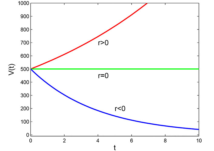
Graph of Malthusian model with initial volume V = 5 × 10^–4 m³

Note. Reprinted from “Mathematical Modelling of the Dynamics of Tumor Growth and its Optimal Control” by Ira JI, Islam MS, Misra JC, Kamrujjaman M. Int J Ground Sediment Water. 2020;11:659–79. (https://www.preprints.org/manuscript/202004.0391/v2). CC BY.

Power law model

The power law model is a generalization of the Malthusian model and was following by Li et al. [15]. This model considers that the rate of tumor growth is not constant, but it changes as the tumor becomes larger. The model shows that the tumor volume increases at a rate proportional to power of the tumor volume itself. This power is denoted by the parameter μ, which is often referred to as the growth exponent. The power law model is a more realistic representation of tumor growth than the exponential model, as it takes into account the fact that tumor growth is not constant.

\frac{d V}{d t} = r V^{b}

Where r is the intrinsic growth rate, if b = 1, we get the Malthusian model which we have already discussed. This equation has the solution of the following form:

V (t) = {[V_{0}^{1 - b} + r (1 - b x (t - t_{0}))]}^{1 / b - 1}

Now we can draw the graph from this solution using different values of b. For b = 1, we get the Malthusian model (Figure 2).

Display full size

Figure 2.

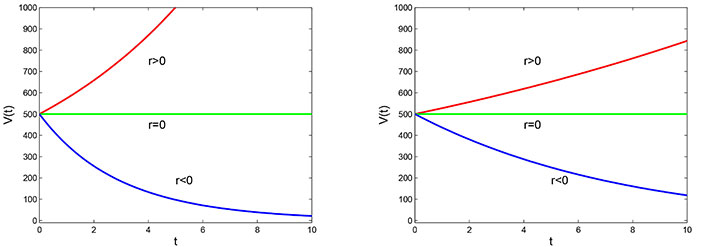
Power law model with initial volume V₀ = 5 × 10^–4 m³ and the exponent, b = 1.05 (left) and b = 0.9 (right)

By observing the graphs of the power law model in Figure 2 with different values of the parameter b, it can be concluded that the behavior of the model changes with different values of b. For instance, when b = 1.05, the tumor volume grows at a faster rate for r > 0 and decays at a faster rate for r < 0. However, when b = 0.9, the growth rate of the tumor volume is slower as compared to the other graph. This indicates that the value of the parameter b has a significant impact on the behavior of the power law model, and its selection should be made carefully depending on the context of the problem being modeled.

Migration model

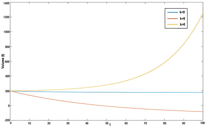
The migration model is a type of mathematical model that describes how a population grows and moves over time. In this model, the growth of the population follows an exponential law, which means that the rate of growth is proportional to the size of the population. The model also takes into account the effect of migration, which can either increase or decrease the population size. When migration occurs, new cells are added to the population, which can increase its size. However, migration can also result in the death of cells, which can reduce the population size. The equation proposed by Murray [12] describes this process mathematically, and it is commonly used in tumor growth research to model the effect of migration on tumor cells.

\frac{d V}{d t} = r V + K

To solve the given equation, the value of r is considered to be zero, and a new variable u is introduced, which is equal to V + K/r. Using this substitution, the given equation can be transformed into a new differential equation that can be solved.

V (t) = (V_{0} + \frac{K}{r}) e^{r (t - t_{0}) - \frac{K}{r}}

This equation shows in Figure 3 the relationship between the tumor volume and time in the presence of migration. If the migration rate K is positive, the tumor volume will increase over time, and if K is negative, the tumor volume will decrease over time.

Display full size

Figure 3.

Graph of Malthusian model with initial volume V = 5 × 10^–4 m³

Gompertz model

The Gompertz model is a mathematical function that describes the growth rate of a tumor. It is a sigmoid function that shows the growth rate is slowest at the beginning and the end of the tumor growth. The model is particularly suitable for modeling breast and lung cancer growth. It has been modified for use in biological populations. The equation of the Gompertz model is a differential equation that is dependent on the growth rate and the carrying capacity of the system. The carrying capacity represents the maximum number of cells that the system can sustain. The Gompertz model is widely used in cancer research to predict tumor growth and to design optimal treatment strategies. The model can be described by the following form Li et al. [15]:

\frac{d V}{d t} = {a e}^{- β t} V

Where a is the intrinsic growth parameter and β is the parameter of growth declaration Integrating both sides by taking limits from V to V and t to t, we get:

V (t) = {V_{0} e}^{\frac{α}{β} (e^{- {β t}_{0}} - e^{- β t})}

For t₀ = 0 the graph of this model is shown in Figure 4.

Display full size

Figure 4.

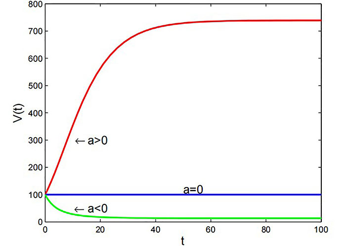
Graph of Gompertz model with β = 1 × 10^–7 m³·day^–1 and V₀ = 10^–4 m³

The Figure 4 shows that when the growth rate a > 0, the tumor volume increases exponentially with time. On the other hand, if the growth rate a < 0, the tumor volume decreases exponentially over time. When the growth rate is equal to 0, the tumor volume remains constant over time.

Logistic model

The logistic equation is a model that takes into account the limited availability of resources for tumor growth, which eventually leads to a saturation point. This model considers that as the tumor grows, there will be competition for essential growth factors like nutrients and space. However, it does not consider the variability of these resources depending on the location of the cells within the tumor. The equation is represented by v(t) for the volume of a solid tumor at time t and a as the proliferation rate of cells.

\frac{d ν}{d t} = λ ν (1 - \frac{ν}{c})

With v(t = 0) = v₀, where c > 0 is the carrying capacity of the environment.

Generalized logistic model

The logistic equation can be extended to include factors such as cell migration, immune response, and drug treatment by adding additional terms to the original equation. The generalized form of the logistic equation Tsoularis and Wallace [9] includes terms that account for the effects of these factors on tumor growth. This form of the equation can be used to model more complex scenarios where these additional factors are present.

\frac{d V}{d t} = a V^{α} {[1 - {(\frac{V}{K})}^{β}]}^{γ}

The generalized form of the logistic equation involves three non-negative exponents α, β, and γ, along with the growth rate parameter α. This equation can be used to derive all the other models described previously by selecting appropriate values for α, β, and γ. For α = 1 and γ = 0, one gets the exponential growth equation by:

\frac{d V}{d t} = a V

The graph of its solution behaves exactly like the exponential growth curve that increases in an unbounded manner, as t → ∞ for α > 0. For α = 1, β = 1, and γ = 1, reduces to the general logistic equation:

\frac{d V}{d t} = a V [1 - (\frac{V}{K})]

The logistic curve can also be generated by setting all the exponents equal to 1. The graph is stable at:

V = \frac{K}{2}

For different initial volumes. If we take α = 2/3, β = 1/3, and γ = 1 we get from general logistic growth equation:

\frac{d V}{d t} = a V^{2 / 3} [1 - {(\frac{V}{K})}^{1 / 3}]

Which is the equation of Von Bertalanffy’s model. We can observe that Von Bertalanffy’s curve gets stable at a slower rate than the logistic curve. Lastly, we can consider α = 1, and γ = 1. Then we get Richard’s equation:

\frac{d V}{d t} = a V [1 - {(\frac{V}{K})}^{β}]

The graph of its solution becomes stable at a faster speed than the normal logistic equation with the smallest increment of β in Figure 5.

Display full size

Figure 5.

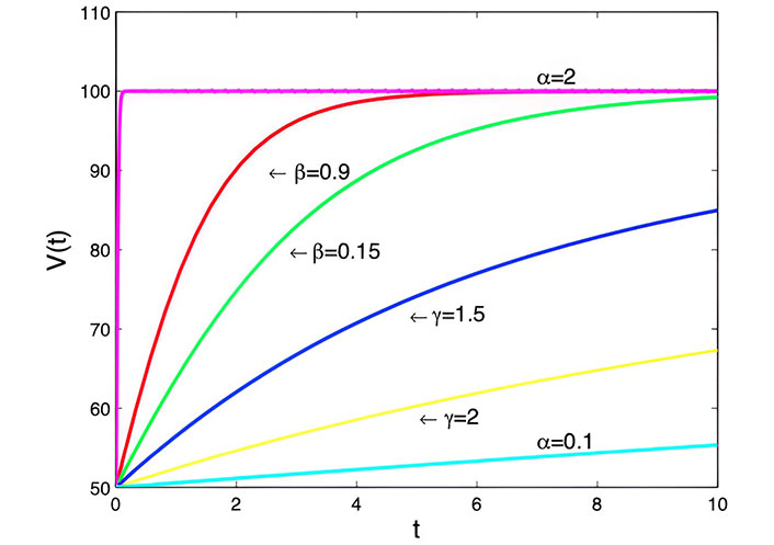
Generalized logistic model with α = 3 cm³·day^–1, K = 100, V = 50 cm³ and t = 0 days to t = 10 days

Von Bertalanffy model

The surface rule model assumes that the growth of a tumor is proportional to its surface area because the nutrients required for growth enter the tumor through its surface. The model also assumes that the rate of cell death is proportional to the tumor size. This model has been used by Tsoularis and Wallace [9] to effectively describe the growth of human tumors.

\frac{d V}{d t} = a V^{2 / 3} - b V

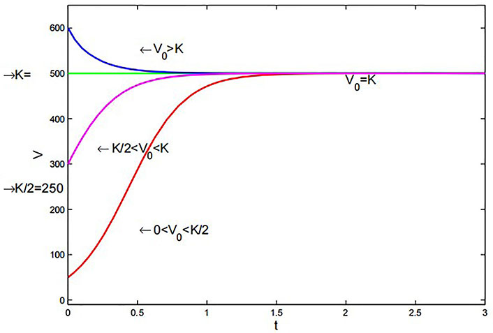
Where a is the growth parameter and b is the growth deceleration parameter. According to Figure 6 solution is given by:

V (t) = {[\frac{a}{b} + ({V_{0}}^{1 / 3} - \frac{a}{b}) e^{- \frac{b}{3} (t - t_{0})}]}^{3}

Display full size

Figure 6.

Graph of Von Bertalanffy model with t₀= 0 days, a = 1.6 × 10^–7 m³·day^–1, b = 0.2 × 10^–7 m³·day^–1, and $K = \frac{a}{b}$

Taking the initial cell volume between 0 and ${(\frac{a}{b})}^{3}$ the cell volume increases over time and gets stable at ${V = (\frac{a}{b})}^{3}$ . Hence, ${V = (\frac{a}{b})}^{3}$ is the saturation level of the model. If we take the initial volume ${V_{0} > (\frac{a}{b})}^{3}$ the volume reduces exponentially over time and is stable at ${V = (\frac{a}{b})}^{3}$ . Also, if we take ${V = (\frac{a}{b})}^{3}$ the volume remains constant.

Richards’ model

The logistic equation was originally designed to describe population growth, but it has also been applied to tumor growth modeling. The Tsoularis and Wallace [9] paper presents the mathematical representation of this model.

\frac{d V}{d t} = a V [1 - {(\frac{V}{K})}^{α}]

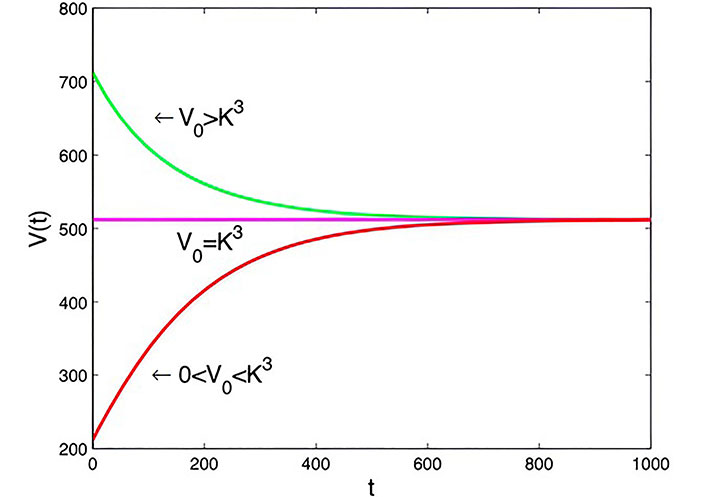
Here α is the positive exponent. We can analytically derive the solution of the above equation by letting $\frac{V^{α - 1}}{K^{α}} = U$ and by using the partial fraction $\frac{1}{V [1 - (\frac{V}{K}) α]} = \frac{1}{V} + \frac{V^{α - 1}}{K^{α} [1 - (\frac{V}{K}) α]}$ . Using these in the equation and integrating both sides we obtain the solution:

V (t) = \frac{K}{{[1 + \{{(\frac{K}{V_{0}})}^{α} - 1\} e^{- a α (t - t_{0})}]}^{1 / α}}

Similar to the logistic model, this model exhibits comparable behavior. However, by adjusting the value of α appropriately in Figure 7, the system can achieve stability faster than the logistic model.

Display full size

Figure 7.

Richards’ model for various initial volumes with a = 5 × 10^–7 m³·day^–1, b = 0.1 × 10^–7 m³·day^–1, α = 1.001, and $K = \frac{a}{b}$

Time-delay model

A time delay refers to a phenomenon where there is a delay or shift in the effect of an input on the resulting output dynamic response, typically in the context of a first-order linear system that incorporates a delay in its feedback mechanism.

Temporal model

One of the classic methods to model tumor growth is by employing differential equations to describe the total number of cells. This approach disregards the spatial characteristics of the cancerous growth.

\frac{d n}{d t} = λ n

Where n represents the number of tumor cells at time t, and λ is the proliferation rate of the tumor, which can be expressed in the form mentioned earlier.

n = n_{0} e^{λ t}

Here n = n₀, is an initial tumor cell. This model assumes that the tumor grows exponentially at the rate λ, in the absence of treatment.

Delay differential equation model

A delay differential equation is a type of mathematical equation where the rate of change of a variable at a certain time point depends not only on its current value but also on its past values, up to a certain time delay. In the context of modeling heterogeneous tumor growth, this time delay factor can be taken into account to capture the effect of spatial heterogeneity and other factors that may affect tumor growth over time. Here, time delay factor (τ units of time). Models of heterogeneous tumor growth:

\frac{d n}{d t} = α n [1 - \frac{n (t - τ)}{c}]

Where n is the number of tumor cells, a is the growth rate, and c is the maximum carrying capacity for tumor cells.

Spatio-temporal model

In the avascular tumor model, the shape of the tumor is assumed to be spherical. To describe this model, Murray [12] developed a density equation, which relates the growth rate of the tumor to the distribution of nutrients in the surrounding tissue. This equation is used to analyze how the growth of the tumor is influenced by factors such as the diffusion of nutrients and the consumption of oxygen.

The rate of change of tumor cell population = the diffusion (motility) of tumor cells + the net proliferation of tumor cells.

\frac{d c}{d t} = \nabla (D \nabla c) + λ c

Where c (x,t) designates the tumor cell density at x radial distance from the origin at time t, and λ is the proliferation rate, and $\nabla$ defines the spatial gradient operator, D is the diffusion coefficient representing the active motility of tumor cells.

c (x, t) = \frac{N_{0} e^{λ (t_{0} + T)} e^{- x^{2 / 4 D t_{0}}}}{8 {(π D t_{0})}^{3 / 2}}

Initially, the tumor cell density is:

c (x, 0) = \frac{N_{0} e^{λ (t_{0})} e^{- x^{2 / 4 D t_{0}}}}{8 {(π D t_{0})}^{3 / 2}}

Heterogeneous model

The previous models assumed that all cells in a tumor are identical, but in reality, tumor cells can differ from one another. To account for this, cells can be divided into three types: proliferating cells, quiescent cells, and necrotic cells. The cells can change their state based on the local conditions, so that proliferating cells can become quiescent or necrotic cells, and quiescent cells can become proliferating or necrotic cells. This modeling approach allows for a more realistic representation of tumor behavior and can help to better understand tumor growth and response to treatment.

Model of heterogeneous tumor growth

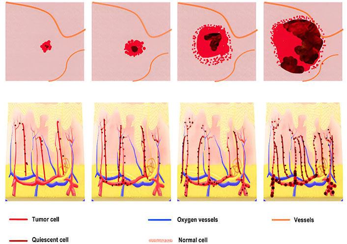
During the tumor growth process, cells in proximity to blood vessels benefit from enhanced nutrient access, resulting in a higher rate of proliferation. Conversely, moving away from blood vessels entails a diminishing nutrient concentration due to consumption and diffusion. Consequently, a region emerges where cells receive just enough nutrients to survive without increasing, forming a quiescent layer. Further distancing from blood vessels leads to a nutrient concentration incapable of sustaining cell survival, resulting in necrosis and subsequent degradation of cells. This progression is visually depicted in a diagram illustrating the transitions between cell states, proliferation, and cell degradation. It’s important to acknowledge that in reality, these state changes are influenced by diverse environmental factors and may occur simultaneously in different tumor regions.

If P(t), is the number of proliferating cells Q(t), is the number of quiescent cells D(t), is the number of necrotic cells at a time. Then the total number of tumor cells N(t), is the sum of all three types of cells that are given by:

N (t) = P (t) + Q (t) + D (t)

From the Figure 8, the following functions:

$M_{α}$ , shows the rate at which proliferating cells produce new cells.
$M_{β}$ , the rate at which the quiescent cells become proliferating.
$M_{γ}$ , the rate at which the proliferating cells become quiescent.
$Z$ , the rate at which the proliferating cells die.
$L$ , the rate at which the quiescent cells die, and λ is the decay rate of the necrotic core. So, a mathematical model can be written as:

\frac{d P}{d t} = (M_{α} - M_{β} - Z) P + M_{β} Q

\frac{d Q}{d t} = M_{γ} P - (M_{β} + L) Q

\frac{d D}{d t} = M_{γ} P - L Q - λ D

Display full size

Figure 8.

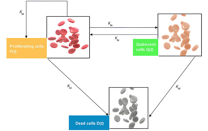
Schematic figure of the model of heterogeneous tumor growth. K_pp represents the rate of cell birth, K_pd is the death rate of proliferating cells, K_pq the rate at which proliferating cells become quiescent and K_qp describes the transformation of Q to P, and K_qd is the rate death of quiescent cells

With the initial conditions as P(0) = P₀, Q(0) = Q₀, and D(0) = D₀.

Angiogenesis and vascular growth model

The model successfully predicted the emergence of distinct regions within a tumor, including a necrotic core, a proliferating rim, and a quiescent region in the middle. Additionally, it considered the impact of anti-angiogenic factors, which could induce tumor size regression by prompting the regression of the capillary network. The methodology involved the integration of two domains: the solid tumor and the surrounding host tissue, and the vasculature domain. The vasculature domain was discretized using a 1D grid that evolved in a Lagrangian manner through the convected element method. Figure 9 shows that communication between the two domains occurred through source and sink terms. The tissue featured a capillary network with a heterogeneous distribution based on a triangular sub-structure. This network evolved dependent on the production and diffusion of Vascular Endothelial Growth Factor (VEGF), Angiopoietin-1, and Angiopoietin-2 along with the presence of related receptors, activating new sides of the triangular mesh accordingly.

Display full size

Figure 9.

Model of vascular and angiogenesis tumor growth

Immunology model

The immune system is a complex network of cells, tissues, and organs that work together to identify and destroy foreign invaders while leaving healthy cells alone. It includes various types of white blood cells, such as T cells, B cells, and natural killer (NK) cells, as well as other specialized cells and molecules. Immunology also involves the study of immune disorders, such as allergies, autoimmune diseases, and immunodeficiencies, which occur when the immune system fails to function properly. Understanding immunology is important for the development of vaccines, immunotherapies, and other treatments for diseases caused by infectious agents or immune disorders.

Immune cell migration model

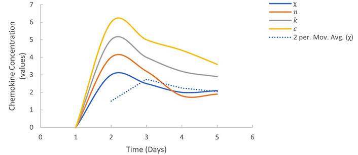
The immune cell migration model is a mathematical model that describes the movement of immune cells, such as T-cells and dendritic cells, toward sites of inflammation or infection. The model assumes that immune cells are attracted to specific chemical signals, known as chemokines, which are produced by cells at the site of infection or inflammation. The model can be described mathematically using partial differential equations, which represent the concentration of chemokines and immune cells over space and time. The equations take into account the diffusion of chemokines and the movement of immune cells towards regions of high chemokine concentration. The equations can be written as follows:

\frac{\partial c}{\partial t} = D \nabla^{2} c - k c

\frac{\partial n}{\partial t} = D_{n} \nabla^{2} n + χ c_{n}

These equations describe how chemokines and immune cells interact in a system. The first equation talks about how chemokines are produced and spread out, but they also degrade over time. The second equation explains how immune cells move towards areas where there are lots of chemokines, with χ representing how sensitive the cells are to these chemical signals. Graphs can help us understand how immune cells move in response to chemokine concentration. The values of the parameters were obtained from Table 1.

Table 1.

Model parameters, descriptions, and values are chosen for simulations

Notation	Value	Description
C	7 × 10^–1	Cancer cells
I	2.1 × 10^–2	Immune system
E	3.8 × 10^–1	Elimination of cancer cells
IC	5.7 × 10^–2	Complex formed between the immune system and cancer cells
c	1 × 10^–7	Concentration of chemokines
n	3.42 × 10^–10	Concentration of immune cells
k	1.8 × 10^–8	Degradation rate of chemokines
D_n	1.3 × 10^–4	Diffusion coefficient of immune cells
t	Est	Time
χ	Est	Sensitivity of immune cells to chemokines
D	4.13 × 10^–2	Diffusion coefficient of chemokines
c_n	5 × 10^–3	Sensitivity of concentration of chemokines

Display full size

Note. Adapted from “Modeling cancer immunoediting in tumor microenvironment with system characterizationthrough the ising-model Hamiltonian” by Rojas-Domínguez A, Arroyo-Duarte R, Rincón-Vieyra F, Alvarado-Mentado M. BMC Bioinformatics. 2022;30:200. (https://bmcbioinformatics.biomedcentral.com/articles/10.1186/s12859-022-04731-w#citeas). CC BY.

The variation in chemokine concentration over time and distance illustrates in the Figure 10 diminishing concentration as it diffuses away from the infection or inflammation source. Meanwhile, a graphical representation of immune cell concentration over time and distance showcases the migration of immune cells towards areas with elevated chemokine concentration, ultimately accumulating at the infection or inflammation site. The immune cell migration model serves as a valuable framework for comprehending the dynamics of immune cell movement towards infection or inflammation sites, offering insights into how factors like chemokine concentration and immune cell sensitivity can influence this process.

Display full size

Figure 10.

Chemokines Immune Cell migration model (2 period moving average)

Cancer immunoediting model

The cancer immunoediting model describes the dynamic relationship between the immune system and cancer cells during tumor development. The model consists of three phases: elimination, equilibrium, and escape. The probability density visualizations in Figures 11, 12, and 13 offer a representation of the energy distribution during the latter phase of the simulations. Instead of depicting the system’s temporal dynamics, these plots encapsulate the system’s energy in a stabilized state.

Display full size

Figure 11.

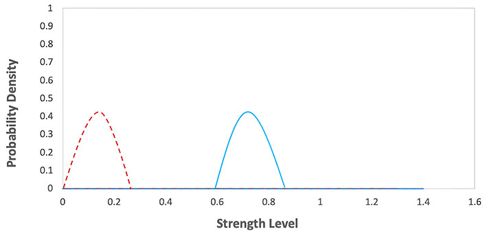
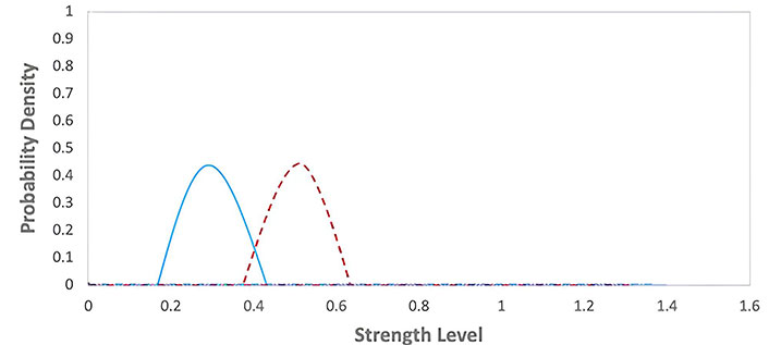
Elimination phase of the immunoediting model. The graph represents the probability density functions for two different groups during an elimination phase, with strength level on the x-axis and probability density on the y-axis. The red dashed line corresponds to the first group with lower strength levels, while the blue solid line corresponds to the second group with higher strength levels

Display full size

Figure 12.

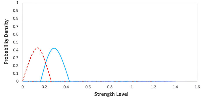
Equilibrium phase of the immunoediting model. The graph represents the probability density functions for two different groups during an equilibrium phase, with strength level on the x-axis and probability density on the y-axis. The red dashed line corresponds to the first group with lower strength levels, while the blue solid line corresponds to the second group with moderately higher strength levels

Display full size

Figure 13.

Escape phase of the immunoediting model table [1]. The graph represents the probability density functions for two different groups during an E phase, with strength level on the x-axis and probability density on the y-axis. The red dashed line corresponds to the first group with lower strength levels, while the blue solid line corresponds to the second group with moderately higher strength levels

Elimination phase: the immune system recognizes and eliminates cancer cells. The equation can represent this:

Immune system (I) + Cancer cells (C) → Elimination of cancer cells

I + C → Elimination of cancer cells

Where I represent the immune system and C represents cancer cells. Immune system attacking and destroying cancer cells. The graph for this phase would show in Figure 11 a decrease in the number of cancer cells over time. The values of the parameters were obtained from Table 1.

Equilibrium phase: The immune system can keep cancer cells in check, preventing them from forming a tumor. A balance between the immune system and cancer cells characterizes this phase.

I + C ↔ IC

Where IC represents the complex formed between the immune system and cancer cells. It represents the equilibrium between the immune system and cancer cells. The graph for this phase would show in Figure 12 a relatively stable number of cancer cells over time, as the immune system can keep the cancer cells. However, cancer cells may acquire mutations that allow them to evade the immune system and progress to the next phase. The values of the parameters were obtained from Table 1.

Escape phase: Cancer cells acquire mutations that allow them to evade the immune system and form a tumor. This phase is characterized by cancer cells escaping immune recognition and attacking, leading to tumor growth and metastasis.

C + I→ Escape

It represents cancer cells escaping immune recognition and attacking. This phase is the most advanced stage of cancer immunoediting and represents the failure of the immune system to control the growth of cancer cells. The graph for this phase would show in Figure 13 a rapid increase in the number of cancer cells over time. The values of the parameters were obtained from Table 1.

The cancer immunoediting model highlights the importance of the immune system in tumor development and provides a framework for understanding how the immune system can be harnessed to treat cancer, such as through immunotherapy. By understanding the different phases of cancer immunoediting, researchers can develop strategies to enhance the immune system’s ability to recognize and eliminate cancer cells or to restore the balance between the immune system and cancer cells in the equilibrium phase.

Results

Begin by introducing the different mathematical models used to study tumor growth dynamics, such as exponential, logistic, time-delay, heterogeneous, and immunology models.

Exponential models

Malthusian model: This model assumes that tumor growth is directly proportional to the number of tumor cells present. When the growth parameter (r) is positive, tumor volume increases exponentially over time, indicating rapid growth. Conversely, when r is negative, tumor volume decreases exponentially, implying decay or treatment effectiveness in Figure 1. A value of zero for r suggests that tumor size remains constant, indicating a balance between growth and decay.

Power law model: Unlike the Malthusian model, the power law model considers that the rate of tumor growth changes as the tumor becomes larger. The parameter ‘b’ determines the nature of tumor growth: if b > 1, the growth rate accelerates with increasing tumor volume, while if 0 < b < 1, growth slows down in Figure 2. This model provides a more realistic representation of tumor growth dynamics.

Migration model: This model incorporates migration effects on tumor growth. A positive migration rate (K) leads to an increase in tumor volume over time as new cells migrate and contribute to growth in Figure 3. Conversely, a negative migration rate results in a decrease in tumor volume, reflecting cell migration away from the tumor.

Gompertz model: The Gompertz model exhibits sigmoidal growth dynamics, reflecting a slow initial growth rate followed by accelerated growth and eventual saturation. Positive growth rates lead to exponential tumor volume increase over time, while negative rates result in exponential decay. When the growth rate equals zero, the tumor volume stabilizes in Figure 4. This model effectively predicts tumor growth characteristics, particularly in breast and lung cancers, aiding in treatment strategy optimization and prognosis assessment.

Logistic models

Generalized logistic model: This model considers the limited availability of resources for tumor growth, leading to a saturation point. The exponents (α, β, and γ) allow for various growth behaviors, influencing the stability and shape of the growth curve in Figure 5. It’s a versatile model capable of representing different growth scenarios.

Von Bertalanffy model: It accounts for the relationship between tumor growth and its surface area, with the rate of cell death proportional to tumor size in Figure 6. The model reaches stability at a saturation level, providing insights into tumor growth dynamics under different conditions.

Richards’ model: Similar to the logistic model, but with an adjustable exponent (α) allowing for faster stability in Figure 7. It offers flexibility in capturing tumor growth patterns with different parameters.

Time-delay models

Temporal model: This model describes tumor growth over time without considering spatial characteristics. It assumes exponential growth in the absence of treatment, providing a basic understanding of tumor dynamics.

Delay differential equation model: By incorporating time delays, this model captures spatial heterogeneity and other factors affecting tumor growth. It offers a more comprehensive representation of tumor behavior over time.

Heterogeneous models

Model of heterogeneous tumor growth: By considering different types of tumor cells (proliferating, quiescent, necrotic), this model offers a more realistic depiction of tumor behavior in Figure 8. It accounts for spatial variations in cell states, providing insights into tumor progression and response to treatment.

Angiogenesis and vascular growth model: This model predicts distinct regions within a tumor and considers the impact of anti-angiogenic factors on tumor regression in Figure 9. It integrates solid tumor and vascular domains to analyze tumor growth dynamics comprehensively.

Immunology models

Immune cell migration model: Describes the movement of immune cells towards infection or inflammation sites based on chemotactic sensitivity in Figure 10. It illustrates how immune cells respond to chemical signals, aiding in the understanding of immune system dynamics.

Cancer immunoediting model: This model highlights the dynamic interaction between the immune system and cancer cells during tumor development in Figures 11, 12, and 13. It emphasizes the role of the immune system in controlling cancer growth and progression through different phases, providing insights into potential immunotherapy strategies.

Each of these models contributes to our understanding of tumor growth and the immune response, offering valuable insights for cancer research and treatment development. By considering various factors such as growth parameters, migration effects, and immune system interactions, these models provide a comprehensive framework for studying tumor dynamics in different contexts.

Discussion

We have explored various mathematical models to study tumor growth and analyzed their effectiveness in predicting the behavior of tumor cells. In addition to the traditional exponential and logistic models, we have also investigated the reaction-diffusion model using a one-dimensional equation and studied the impact of heterogeneity and time delay on tumor growth. we have incorporated the immune system into our models to explore its impact on tumor growth and found that it plays a crucial role in controlling tumor cell proliferation. We have also developed a model to investigate the optimal control in the case of chemotherapy and analyzed its effectiveness in reducing tumor cell volume. Through our numerical analysis using the Finite difference method, we have observed that the initial location of a tumor and the diffusion coefficients are critical factors in predicting tumor growth. Furthermore, we have demonstrated the potential of mathematical modeling in predicting tumor growth without the need for laboratory tests. Overall, our study highlights the significance of interdisciplinary research between Mathematics and Biology in advancing our understanding of tumor growth and developing effective strategies for cancer treatment.

Declarations

Acknowledgments

This work is supported under a research project entitled “Mathematical modeling of tumor growth and its treatments” granted by the U.P. State Government under the supervision of Prof. Sanjeev Kumar.

Author contributions

DG: Conceptualization, Methodology, Formal analysis, Investigation, Visualization, Writing—original draft. SK: Conceptualization, Writing—review & editing, Supervision. RS: Data curation. DD: Validation, Writing—review & editing.

Conflicts of interest

The authors declare that they have no conflicts of interest.

Ethical approval

Not applicable.

Consent to participate

Not applicable.

Consent to publication

Not applicable.

Availability of data and materials

The datasets that support the findings of this study are available from the corresponding author upon reasonable request.

Funding

Not applicable.

Copyright

References

Gompertz B. On the nature of the function expressive of the law of human mortality, and on a new mode of determining the value of life contingencies. Philos Trans R Soc Lond. 1825;115:513–83. [DOI]

Winsor CP. The Gompertz Curve as a Growth Curve. Proc Natl Acad Sci U S A. 1932;18:1–8. [DOI] [PubMed] [PMC]

Laird AK, Tyler SA, Barton AD. Dynamics of normal growth. Growth. 1965;29:233–48. [PubMed]

Burton AC. Rate of growth of solid tumours as a problem of diffusion. Growth. 1966;30:157–76. [PubMed]

Orme ME, Chaplain MAJ. A mathematical model of vascular tumour growth and invasion. Math Comput Modell. 1996;23:43–60. [DOI]

Anderson AR, Chaplain MA. Continuous and discrete mathematical models of tumor-induced angiogenesis. Bull Math Biol. 1998;60:857–99. [DOI] [PubMed]

Bellomo N, Preziosi L. Modelling and mathematical problems related to tumor evolution and its interaction with the immune system. Math Comput Modell. 2000;32:413–52. [DOI]

Sherratt JA, Chaplain MA. A new mathematical model for avascular tumour growth. J Math Biol. 2001;43:291–312. [DOI] [PubMed]

Tsoularis A, Wallace J. Analysis of logistic growth models. Math Biosci. 2002;179:21–55. [DOI] [PubMed]

10.

Villasana M, Radunskaya A. A delay differential equation model for tumor growth. J Math Biol. 2003;47:270–94. [DOI] [PubMed]

11.

Misra JC, Dravid B. A mathematical model in the study of genes for identifying transcription factor binding sites. Comput Math Appl. 2006;51:621–30. [DOI]

12.

Murray JD. Mathematical Biology: I. An Introduction. 3rd ed. Springer-Verlag Berlin Heidelberg; 2002.

13.

Yang HM. Mathematical modeling of solid cancer growth with angiogenesis. Theor Biol Med Model. 2012;9:2. [DOI] [PubMed] [PMC]

14.

Dixit DS, Kumar D, Kumar S, Johri R. Mathematical Modelling For Chemotherapy Of Tumor Growth With Aspect Of Biological Stoichiometry. Global J Pure Appl Math. 2015;11:2581–7.

15.

Li Y, Cheng H, Wang J, Wang Y. Dynamic analysis of unilateral diffusion Gompertz model with impulsive control strategy. Adv Differ Equ. 2018:32. [DOI]

16.

Wei HC. A mathematical model of tumour growth with Beddington-DeAngelis functional response: a case of cancer without disease. J Biol Dyn. 2018;12:194–210. [DOI] [PubMed]

17.

Yin A, Moes DJAR, van Hasselt JGC, Swen JJ, Guchelaar HJ. A Review of Mathematical Models for Tumor Dynamics and Treatment Resistance Evolution of Solid Tumors. CPT Pharmacometrics Syst Pharmacol. 2019;8:720–37. [DOI] [PubMed] [PMC]

18.

Ira JI, Islam MS, Misra JC, Kamrujjaman M. Mathematical Modelling of the Dynamics of Tumor Growth and its Optimal Control. Int J Ground Sediment Water. 2020;11:659–79. [DOI]

19.

Pourhasanzade F, Sabzpoushan SH. A New Mathematical Model for Controlling Tumor Growth Based on Microenvironment Acidity and Oxygen Concentration. Biomed Res Int. 2021;2021:8886050. [DOI] [PubMed] [PMC]

20.

Rojas-Domínguez A, Arroyo-Duarte R, Rincón-Vieyra F, Alvarado-Mentado M. Modeling cancer immunoediting in tumor microenvironment with system characterization through the ising-model Hamiltonian. BMC Bioinformatics. 2022;23:200. [DOI] [PubMed] [PMC]

21.

Ullah MA, Mallick UK. Mathematical Modeling and Analysis on the Effects of Surgery and Chemotherapy on Lung Cancer. J Appl Math. 2023;2023:1–16. [DOI]

22.

Wei K, Du Z, Deng J, Yang J, Chen H. A Novel Pyroptosis-Based Prognostic Model Correlated with the Parainflammatory Immune Microenvironment of Pancreatic Cancer. J Appl Math. 2023;2023:1–26. [DOI]